Choose a dataset and one of its held-out test cases, then compare the trained surrogates side by side with the finite-element (FEM) result and a pixel-wise error map. Or set up a new case of your own: the surrogates then run live in your browser.
Phase-field models are the method of choice for simulating fracture (crack nucleation, propagation, branching and coalescence) within a single variational framework. But each quasi-static simulation is expensive, which makes ensemble workflows such as uncertainty quantification, Bayesian inference and design optimization intractable.
Fracture-Bench is a benchmark suite that evaluates machine-learning surrogates which replace the finite-element solve with a single network forward pass. Five architectures (UNet, FNO, DeepONet, Latent DeepONet and a conditional denoising diffusion model) are trained on identical data splits and scored with common test metrics across two high-fidelity datasets that differ in phase-field formulation, material heterogeneity and prediction task.
Evaluation spans accuracy, computational efficiency and generalization to load steps withheld during training. The headline result: no single architecture dominates, and prediction difficulty grows with material heterogeneity and crack-path sensitivity. The datasets, evaluation protocols and model code are released openly.
Dataset 1 : Perforated plate of hyperelastic material
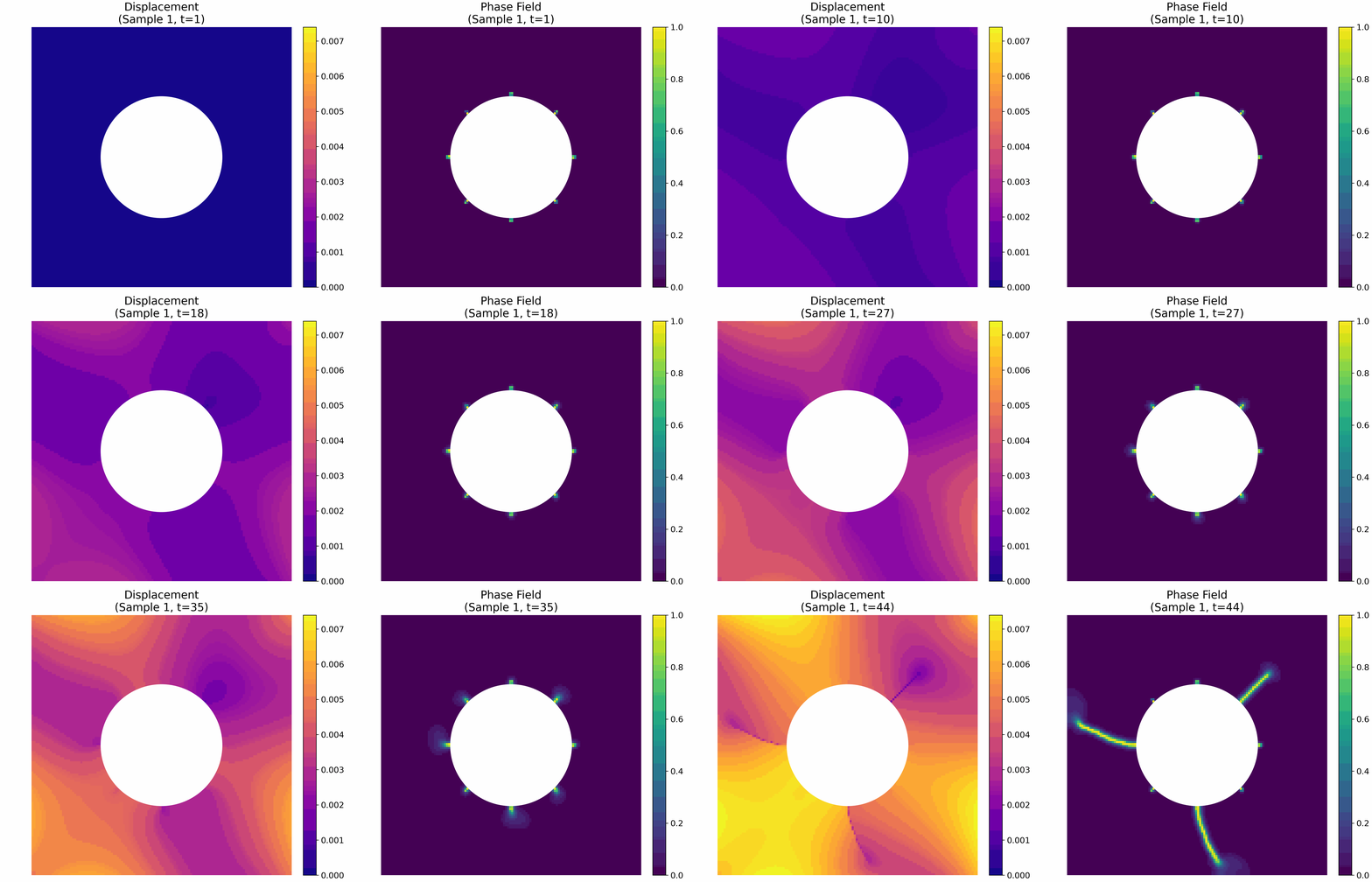
- Formulation: phase-field fracture, AT2 model
- Domain: Ω = [−1.1, 1.1]² square plate, central hole r = 0.5, eight notches · grid 128 × 128
- Loading: boundary displacement u = ε̄n f(s) x on ∂Ω, with f a periodic Gaussian random field · 44 load steps
- Operator: 𝒢 : u(x,0) ↦ d(x,t), t ∈ {t1,…,t44}
- Phase field: vector d(x,t) ∈ ℝ² (after Hakimzadeh et al.); the scalar damage ‖d‖ ∈ [0,1] is shown
- Size: 1,000 simulations · train / test = 900 / 100
- Download the full dataset from the JHU Data Archive.
- Get the simulation and data-generation code from the GitHub repository.
- See how the crack path changes with the boundary load:
Dataset 2 : Heterogeneous plate with two inclusions
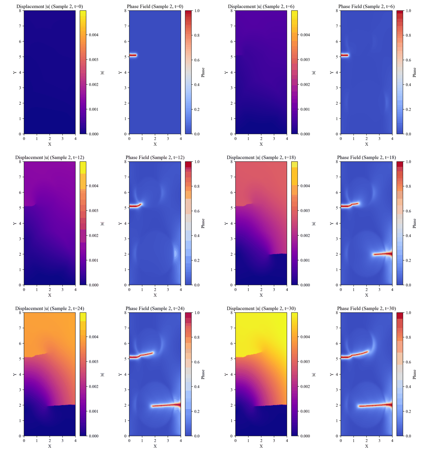
- Formulation: phase-field fracture, PF-CZM model
- Domain: 4 mm × 8 mm plate · two circular inclusions · grid 128 × 256
- Material: modulus field E(x); each inclusion stiffer (E = 10 Em) or softer (E = 0.1 Em) than the matrix
- Loading: Mode-I tension, 31 load steps
- Operator: 𝒢 : (d(x,0), E(x)) ↦ d(x,tf)
- Phase field: scalar d ∈ [0,1] (0 = intact, 1 = fully cracked); only the final step tf is predicted
- Size: 4,000 simulations (4 inclusion configurations) · train / test = 3,600 / 400
- Download the full dataset from the JHU Data Archive.
- Get the adaptive-mesh simulation and data-generation code from the GitHub repository.
- See how the crack path bends around the inclusions:
Contributing & contact
Fracture-Bench is meant to grow as a community resource. If you would like to contribute a new surrogate architecture, or a new dataset or fracture problem, we would be glad to include it. Please reach out to any of us (the full team is listed on the home page):
- Dr. U. Meenu Krishnan · ukrishn4@jh.edu
- Prof. Somdatta Goswami · somdatta@jhu.edu
- Prof. Lori Graham-Brady · lori@jhu.edu
- Test case: one of 10 held-out FEM simulations that the models never saw in training.
- Surrogates: compare FNO, DeepONet and Latent DeepONet at 11, 22 or 44 load steps.
- Output: the damage ‖d(x,t)‖ at each load step next to FEM, and the error |prediction − FEM| below. Press Play to watch the crack grow.
- New load: switch the input to New load (live) to draw your own boundary load. DeepONet and Latent DeepONet then predict the crack growth in your browser.
Boundary load
A new load from the Gaussian random field of the FEM data generator:
f(s) = μ + Σn λn [ξn cos nφ + ηn sin nφ], λn = √2 σ ((2πn)² + τ²)−γ/2
The training data used γ = 4, τ = 5, σ = 625 and μ = 1. Other values give loads unlike any the model was trained on.
Surrogates
FNO is not offered here: its Dataset 1 models (1.2 GB each) are too large for a browser. Compare it on the held-out test cases.
‖d(x, t)‖: predictions
Choose the surrogates and press Predict crack evolution.
The models run on your computer with the trained weights. Each model is downloaded once; its size is shown next to its name. A prediction takes about a second on a laptop, a little longer at 44 load steps. A new load has no FEM result, so there is no error map. The 44-step DeepONet comes from a supplementary run.
Input
Surrogates
UNet and cDDPM will be added once their trained weights are released.
‖d(x, t)‖: prediction and FEM
|prediction − FEM|
Predictions were computed once with the trained models. The error scale is capped at the 95th percentile of the errors at each load step. MSE is the mean squared error of ‖d‖ at the shown step, outside the hole. The 11- and 22-step FNO models are re-runs that saved their spectral weights, and the 44-step DeepONet comes from a supplementary run (in the paper, that configuration did not reach the error threshold).
- Test case: one of 10 held-out FEM simulations covering all four inclusion configurations.
- Surrogates: compare FNO, DeepONet and Latent DeepONet.
- Output: the phase field d(x,tf) at the final load step next to FEM, and the error |prediction − FEM| below.
- Your own setup: switch the input to Custom setup (live) to choose the inclusions and place the initial crack. FNO, DeepONet and Latent DeepONet then predict the final crack in your browser.
Inclusions
Initial crack tip
The tip can be placed where the training cracks started. You can also click on the plate below.
- stiffer inclusion (10 Em)
- softer inclusion (0.1 Em)
- initial crack
Surrogates
d(x, tf): predictions
Choose the surrogates and press Predict final crack path.
The models run on your computer with the trained weights. Each model is downloaded once; its size is shown next to its name. The first prediction takes a few seconds; after that, the result updates as you change the setup. A custom setup has no FEM result, so there is no error map.
Input
- stiffer inclusion (10 Em)
- softer inclusion (0.1 Em)
- initial crack
Surrogates
UNet and cDDPM will be added once their trained weights are released.
d(x, tf): prediction and FEM
|prediction − FEM|
Predictions were computed once with the trained models. The error scale is capped at the 95th percentile of the errors. MSE is the mean squared error of d over the whole plate.